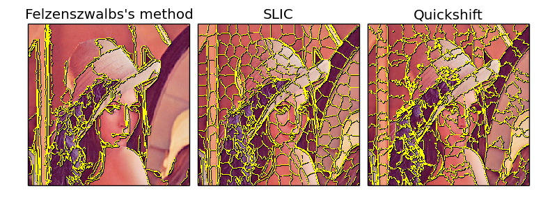
This example compares three popular low-level image segmentation methods. As it is difficult to obtain good segmentations, and the definition of “good” often depends on the application, these methods are usually used for obtaining an oversegmentation, also known as superpixels. These superpixels then serve as a basis for more sophisticated algorithms such as conditional random fields (CRF).
This fast 2D image segmentation algorithm, proposed in [1] is popular in the computer vision community. The algorithm has a single scale parameter that influences the segment size. The actual size and number of segments can vary greatly, depending on local contrast.
| [1] | Efficient graph-based image segmentation, Felzenszwalb, P.F. and Huttenlocher, D.P. International Journal of Computer Vision, 2004 |
Quickshift is a relatively recent 2D image segmentation algorithm, based on an approximation of kernelized mean-shift. Therefore it belongs to the family of local mode-seeking algorithms and is applied to the 5D space consisting of color information and image location [2].
One of the benefits of quickshift is that it actually computes a hierarchical segmentation on multiple scales simultaneously.
Quickshift has two main parameters: sigma controls the scale of the local density approximation, max_dist selects a level in the hierarchical segmentation that is produced. There is also a trade-off between distance in color-space and distance in image-space, given by ratio.
| [2] | Quick shift and kernel methods for mode seeking, Vedaldi, A. and Soatto, S. European Conference on Computer Vision, 2008 |
This algorithm simply performs K-means in the 5d space of color information and image location and is therefore closely related to quickshift. As the clustering method is simpler, it is very efficient. It is essential for this algorithm to work in Lab color space to obtain good results. The algorithm quickly gained momentum and is now widely used. See [3] for details. The compactness parameter trades off color-similarity and proximity, as in the case of Quickshift, while n_segments chooses the number of centers for kmeans.
| [3] | Radhakrishna Achanta, Appu Shaji, Kevin Smith, Aurelien Lucchi, Pascal Fua, and Sabine Suesstrunk, SLIC Superpixels Compared to State-of-the-art Superpixel Methods, TPAMI, May 2012. |
from __future__ import print_function

import matplotlib.pyplot as plt
import numpy as np

from skimage.data import lena
from skimage.segmentation import felzenszwalb, slic, quickshift
from skimage.segmentation import mark_boundaries
from skimage.util import img_as_float

img = img_as_float(lena()[::2, ::2])
segments_fz = felzenszwalb(img, scale=100, sigma=0.5, min_size=50)
segments_slic = slic(img, n_segments=250, compactness=10, sigma=1)
segments_quick = quickshift(img, kernel_size=3, max_dist=6, ratio=0.5)

print("Felzenszwalb's number of segments: %d" % len(np.unique(segments_fz)))
print("Slic number of segments: %d" % len(np.unique(segments_slic)))
print("Quickshift number of segments: %d" % len(np.unique(segments_quick)))

fig, ax = plt.subplots(1, 3)
fig.set_size_inches(8, 3, forward=True)
fig.subplots_adjust(0.05, 0.05, 0.95, 0.95, 0.05, 0.05)

ax[0].imshow(mark_boundaries(img, segments_fz))
ax[0].set_title("Felzenszwalbs's method")
ax[1].imshow(mark_boundaries(img, segments_slic))
ax[1].set_title("SLIC")
ax[2].imshow(mark_boundaries(img, segments_quick))
ax[2].set_title("Quickshift")
for a in ax:
    a.set_xticks(())
    a.set_yticks(())
plt.show()

STDOUT
STDERR
Python source code: download (generated using skimage 0.11dev)
IPython Notebook: download (generated using skimage 0.11dev)