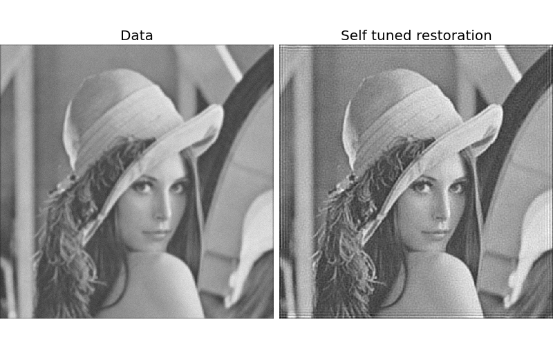
In this example, we deconvolve a noisy version of Lena using Wiener and unsupervised Wiener algorithms. This algorithms are based on linear models that can’t restore sharp edge as much as non-linear methods (like TV restoration) but are much faster.
The inverse filter based on the PSF (Point Spread Function), the prior regularisation (penalisation of high frequency) and the tradeoff between the data and prior adequacy. The regularization parameter must be hand tuned.
This algorithm has a self-tuned regularisation parameters based on data learning. This is not common and based on the following publication. The algorithm is based on a iterative Gibbs sampler that draw alternatively samples of posterior conditionnal law of the image, the noise power and the image frequency power.
| [1] | François Orieux, Jean-François Giovannelli, and Thomas Rodet, “Bayesian estimation of regularization and point spread function parameters for Wiener-Hunt deconvolution”, J. Opt. Soc. Am. A 27, 1593-1607 (2010) |
import numpy as np
import matplotlib.pyplot as plt

from skimage import color, data, restoration

lena = color.rgb2gray(data.lena())
from scipy.signal import convolve2d as conv2
psf = np.ones((5, 5)) / 25
lena = conv2(lena, psf, 'same')
lena += 0.1 * lena.std() * np.random.standard_normal(lena.shape)

deconvolved, _ = restoration.unsupervised_wiener(lena, psf)

fig, ax = plt.subplots(nrows=1, ncols=2, figsize=(8, 5))

plt.gray()

ax[0].imshow(lena, vmin=deconvolved.min(), vmax=deconvolved.max())
ax[0].axis('off')
ax[0].set_title('Data')

ax[1].imshow(deconvolved)
ax[1].axis('off')
ax[1].set_title('Self tuned restoration')

fig.subplots_adjust(wspace=0.02, hspace=0.2,
                    top=0.9, bottom=0.05, left=0, right=1)

plt.show()

STDOUT
STDERR
Python source code: download (generated using skimage 0.11dev)
IPython Notebook: download (generated using skimage 0.11dev)