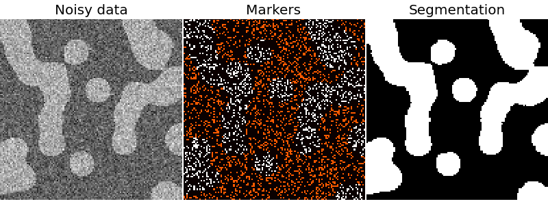
The random walker algorithm [1] determines the segmentation of an image from a set of markers labeling several phases (2 or more). An anisotropic diffusion equation is solved with tracers initiated at the markers’ position. The local diffusivity coefficient is greater if neighboring pixels have similar values, so that diffusion is difficult across high gradients. The label of each unknown pixel is attributed to the label of the known marker that has the highest probability to be reached first during this diffusion process.
In this example, two phases are clearly visible, but the data are too noisy to perform the segmentation from the histogram only. We determine markers of the two phases from the extreme tails of the histogram of gray values, and use the random walker for the segmentation.
| [1] | Random walks for image segmentation, Leo Grady, IEEE Trans. Pattern Anal. Mach. Intell. 2006 Nov; 28(11):1768-83 |
import numpy as np
from scipy import ndimage
import matplotlib.pyplot as plt

from skimage.segmentation import random_walker


def microstructure(l=256):
    """
    Synthetic binary data: binary microstructure with blobs.

    Parameters
    ----------

    l: int, optional
        linear size of the returned image
    """
    n = 5
    x, y = np.ogrid[0:l, 0:l]
    mask = np.zeros((l, l))
    generator = np.random.RandomState(1)
    points = l * generator.rand(2, n ** 2)
    mask[(points[0]).astype(np.int), (points[1]).astype(np.int)] = 1
    mask = ndimage.gaussian_filter(mask, sigma=l / (4. * n))
    return (mask > mask.mean()).astype(np.float)


# Generate noisy synthetic data
data = microstructure(l=128)
data += 0.35 * np.random.randn(*data.shape)
markers = np.zeros(data.shape, dtype=np.uint)
markers[data < -0.3] = 1
markers[data > 1.3] = 2

# Run random walker algorithm
labels = random_walker(data, markers, beta=10, mode='bf')

# Plot results
fig, (ax1, ax2, ax3) = plt.subplots(1, 3, figsize=(8, 3.2))
ax1.imshow(data, cmap='gray', interpolation='nearest')
ax1.axis('off')
ax1.set_title('Noisy data')
ax2.imshow(markers, cmap='hot', interpolation='nearest')
ax2.axis('off')
ax2.set_title('Markers')
ax3.imshow(labels, cmap='gray', interpolation='nearest')
ax3.axis('off')
ax3.set_title('Segmentation')

fig.subplots_adjust(hspace=0.01, wspace=0.01, top=1, bottom=0, left=0,
                    right=1)
plt.show()

STDOUT
STDERR
Python source code: download (generated using skimage 0.11dev)
IPython Notebook: download (generated using skimage 0.11dev)