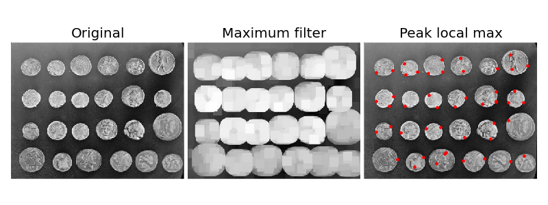
The peak_local_max function returns the coordinates of local peaks (maxima) in an image. A maximum filter is used for finding local maxima. This operation dilates the original image and merges neighboring local maxima closer than the size of the dilation. Locations where the original image is equal to the dilated image are returned as local maxima.
from scipy import ndimage
import matplotlib.pyplot as plt
from skimage.feature import peak_local_max
from skimage import data, img_as_float

im = img_as_float(data.coins())

# image_max is the dilation of im with a 20*20 structuring element
# It is used within peak_local_max function
image_max = ndimage.maximum_filter(im, size=20, mode='constant')

# Comparison between image_max and im to find the coordinates of local maxima
coordinates = peak_local_max(im, min_distance=20)

# display results
fig, ax = plt.subplots(1, 3, figsize=(8, 3))
ax1, ax2, ax3 = ax.ravel()
ax1.imshow(im, cmap=plt.cm.gray)
ax1.axis('off')
ax1.set_title('Original')

ax2.imshow(image_max, cmap=plt.cm.gray)
ax2.axis('off')
ax2.set_title('Maximum filter')

ax3.imshow(im, cmap=plt.cm.gray)
ax3.autoscale(False)
ax3.plot(coordinates[:, 1], coordinates[:, 0], 'r.')
ax3.axis('off')
ax3.set_title('Peak local max')

fig.subplots_adjust(wspace=0.02, hspace=0.02, top=0.9,
                    bottom=0.02, left=0.02, right=0.98)

plt.show()

STDOUT
STDERR
Python source code: download (generated using skimage 0.11dev)
IPython Notebook: download (generated using skimage 0.11dev)