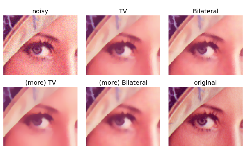
Denoising the picture of Lena
In this example, we denoise a noisy version of the picture of Lena using the total variation and bilateral denoising filter.
These algorithms typically produce “posterized” images with flat domains separated by sharp edges. It is possible to change the degree of posterization by controlling the tradeoff between denoising and faithfulness to the original image.
Total variation filter
The result of this filter is an image that has a minimal total variation norm, while being as close to the initial image as possible. The total variation is the L1 norm of the gradient of the image.
Bilateral filter
A bilateral filter is an edge-preserving and noise reducing filter. It averages pixels based on their spatial closeness and radiometric similarity.

import numpy as np
import matplotlib.pyplot as plt

from skimage import data, img_as_float
from skimage.restoration import denoise_tv_chambolle, denoise_bilateral


lena = img_as_float(data.lena())
lena = lena[220:300, 220:320]

noisy = lena + 0.6 * lena.std() * np.random.random(lena.shape)
noisy = np.clip(noisy, 0, 1)

fig, ax = plt.subplots(nrows=2, ncols=3, figsize=(8, 5))

plt.gray()

ax[0, 0].imshow(noisy)
ax[0, 0].axis('off')
ax[0, 0].set_title('noisy')
ax[0, 1].imshow(denoise_tv_chambolle(noisy, weight=0.1, multichannel=True))
ax[0, 1].axis('off')
ax[0, 1].set_title('TV')
ax[0, 2].imshow(denoise_bilateral(noisy, sigma_range=0.05, sigma_spatial=15))
ax[0, 2].axis('off')
ax[0, 2].set_title('Bilateral')

ax[1, 0].imshow(denoise_tv_chambolle(noisy, weight=0.2, multichannel=True))
ax[1, 0].axis('off')
ax[1, 0].set_title('(more) TV')
ax[1, 1].imshow(denoise_bilateral(noisy, sigma_range=0.1, sigma_spatial=15))
ax[1, 1].axis('off')
ax[1, 1].set_title('(more) Bilateral')
ax[1, 2].imshow(lena)
ax[1, 2].axis('off')
ax[1, 2].set_title('original')

fig.subplots_adjust(wspace=0.02, hspace=0.2,
                    top=0.9, bottom=0.05, left=0, right=1)

plt.show()

STDOUT
STDERR
Python source code: download (generated using skimage 0.11dev)
IPython Notebook: download (generated using skimage 0.11dev)
