In this example, we will see how to segment objects from a background. We use the coins image from skimage.data, which shows several coins outlined against a darker background.
import numpy as np
import matplotlib.pyplot as plt

from skimage import data

coins = data.coins()
hist = np.histogram(coins, bins=np.arange(0, 256))

fig, (ax1, ax2) = plt.subplots(1, 2, figsize=(8, 3))
ax1.imshow(coins, cmap=plt.cm.gray, interpolation='nearest')
ax1.axis('off')
ax2.plot(hist[1][:-1], hist[0], lw=2)
ax2.set_title('histogram of grey values')

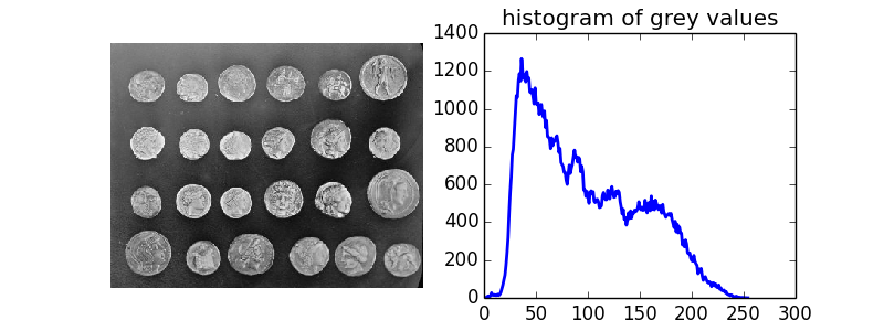
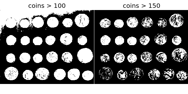
A simple way to segment the coins is to choose a threshold based on the histogram of grey values. Unfortunately, thresholding this image gives a binary image that either misses significant parts of the coins or merges parts of the background with the coins:
fig, (ax1, ax2) = plt.subplots(1, 2, figsize=(6, 3))
ax1.imshow(coins > 100, cmap=plt.cm.gray, interpolation='nearest')
ax1.set_title('coins > 100')
ax1.axis('off')
ax2.imshow(coins > 150, cmap=plt.cm.gray, interpolation='nearest')
ax2.set_title('coins > 150')
ax2.axis('off')
margins = dict(hspace=0.01, wspace=0.01, top=1, bottom=0, left=0, right=1)
fig.subplots_adjust(**margins)
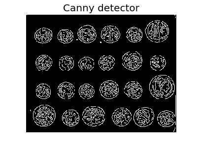
Next, we try to delineate the contours of the coins using edge-based segmentation. To do this, we first get the edges of features using the Canny edge-detector.
from skimage.filter import canny
edges = canny(coins/255.)

fig, ax = plt.subplots(figsize=(4, 3))
ax.imshow(edges, cmap=plt.cm.gray, interpolation='nearest')
ax.axis('off')
ax.set_title('Canny detector')
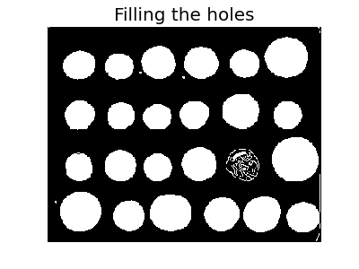
These contours are then filled using mathematical morphology.
from scipy import ndimage

fill_coins = ndimage.binary_fill_holes(edges)

fig, ax = plt.subplots(figsize=(4, 3))
ax.imshow(fill_coins, cmap=plt.cm.gray, interpolation='nearest')
ax.axis('off')
ax.set_title('Filling the holes')
Small spurious objects are easily removed by setting a minimum size for valid objects.
from skimage import morphology
coins_cleaned = morphology.remove_small_objects(fill_coins, 21)

fig, ax = plt.subplots(figsize=(4, 3))
ax.imshow(coins_cleaned, cmap=plt.cm.gray, interpolation='nearest')
ax.axis('off')
ax.set_title('Removing small objects')
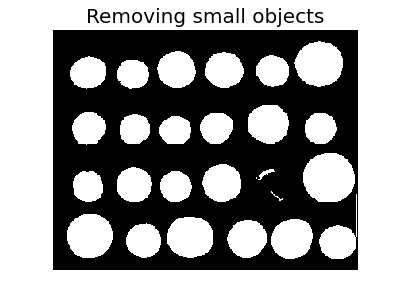
However, this method is not very robust, since contours that are not perfectly closed are not filled correctly, as is the case for one unfilled coin above.
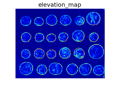
We therefore try a region-based method using the watershed transform. First, we find an elevation map using the Sobel gradient of the image.
from skimage.filter import sobel

elevation_map = sobel(coins)

fig, ax = plt.subplots(figsize=(4, 3))
ax.imshow(elevation_map, cmap=plt.cm.jet, interpolation='nearest')
ax.axis('off')
ax.set_title('elevation_map')
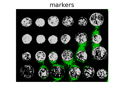
Next we find markers of the background and the coins based on the extreme parts of the histogram of grey values.
markers = np.zeros_like(coins)
markers[coins < 30] = 1
markers[coins > 150] = 2

fig, ax = plt.subplots(figsize=(4, 3))
ax.imshow(markers, cmap=plt.cm.spectral, interpolation='nearest')
ax.axis('off')
ax.set_title('markers')
Finally, we use the watershed transform to fill regions of the elevation map starting from the markers determined above:
segmentation = morphology.watershed(elevation_map, markers)

fig, ax = plt.subplots(figsize=(4, 3))
ax.imshow(segmentation, cmap=plt.cm.gray, interpolation='nearest')
ax.axis('off')
ax.set_title('segmentation')
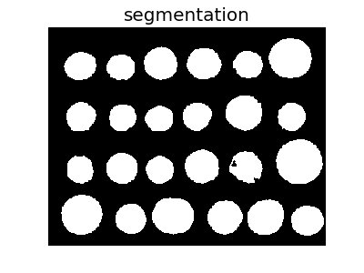
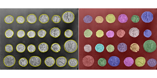
This last method works even better, and the coins can be segmented and labeled individually.
from skimage.color import label2rgb

segmentation = ndimage.binary_fill_holes(segmentation - 1)
labeled_coins, _ = ndimage.label(segmentation)
image_label_overlay = label2rgb(labeled_coins, image=coins)

fig, (ax1, ax2) = plt.subplots(1, 2, figsize=(6, 3))
ax1.imshow(coins, cmap=plt.cm.gray, interpolation='nearest')
ax1.contour(segmentation, [0.5], linewidths=1.2, colors='y')
ax1.axis('off')
ax2.imshow(image_label_overlay, interpolation='nearest')
ax2.axis('off')

fig.subplots_adjust(**margins)
plt.show()
STDOUT
STDERR
Python source code: download (generated using skimage 0.11dev)
IPython Notebook: download (generated using skimage 0.11dev)