Rank filters
Rank filters are non-linear filters using the local gray-level ordering to compute the filtered value. This ensemble of filters share a common base: the local gray-level histogram is computed on the neighborhood of a pixel (defined by a 2-D structuring element). If the filtered value is taken as the middle value of the histogram, we get the classical median filter.
Rank filters can be used for several purposes such as:
- image quality enhancement e.g. image smoothing, sharpening
- image pre-processing e.g. noise reduction, contrast enhancement
- feature extraction e.g. border detection, isolated point detection
- post-processing e.g. small object removal, object grouping, contour smoothing
Some well known filters are specific cases of rank filters [1] e.g. morphological dilation, morphological erosion, median filters.
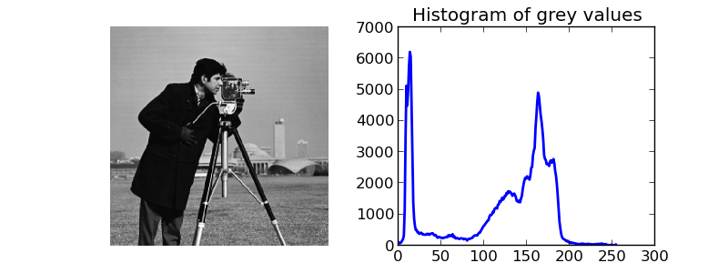
In this example, we will see how to filter a gray-level image using some of the linear and non-linear filters available in skimage. We use the camera image from skimage.data for all comparisons.
| [1] | (1, 2) Pierre Soille, On morphological operators based on rank filters, Pattern Recognition 35 (2002) 527-535. |
import numpy as np
import matplotlib.pyplot as plt

from skimage import img_as_ubyte
from skimage import data

noisy_image = img_as_ubyte(data.camera())
hist = np.histogram(noisy_image, bins=np.arange(0, 256))

fig, (ax1, ax2) = plt.subplots(1, 2, figsize=(8, 3))
ax1.imshow(noisy_image, interpolation='nearest', cmap=plt.cm.gray)
ax1.axis('off')
ax2.plot(hist[1][:-1], hist[0], lw=2)
ax2.set_title('Histogram of grey values')
Noise removal
Some noise is added to the image, 1% of pixels are randomly set to 255, 1% are randomly set to 0. The median filter is applied to remove the noise.
from skimage.filter.rank import median
from skimage.morphology import disk

noise = np.random.random(noisy_image.shape)
noisy_image = img_as_ubyte(data.camera())
noisy_image[noise > 0.99] = 255
noisy_image[noise < 0.01] = 0

fig, ax = plt.subplots(2, 2, figsize=(10, 7))
ax1, ax2, ax3, ax4 = ax.ravel()

ax1.imshow(noisy_image, vmin=0, vmax=255, cmap=plt.cm.gray)
ax1.set_title('Noisy image')
ax1.axis('off')

ax2.imshow(median(noisy_image, disk(1)), vmin=0, vmax=255, cmap=plt.cm.gray)
ax2.set_title('Median $r=1$')
ax2.axis('off')

ax3.imshow(median(noisy_image, disk(5)), vmin=0, vmax=255, cmap=plt.cm.gray)
ax3.set_title('Median $r=5$')
ax3.axis('off')

ax4.imshow(median(noisy_image, disk(20)), vmin=0, vmax=255, cmap=plt.cm.gray)
ax4.set_title('Median $r=20$')
ax4.axis('off')
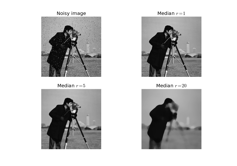
The added noise is efficiently removed, as the image defaults are small (1 pixel wide), a small filter radius is sufficient. As the radius is increasing, objects with bigger sizes are filtered as well, such as the camera tripod. The median filter is often used for noise removal because borders are preserved and e.g. salt and pepper noise typically does not distort the gray-level.
Image smoothing
The example hereunder shows how a local mean filter smooths the camera man image.
from skimage.filter.rank import mean

fig, (ax1, ax2) = plt.subplots(1, 2, figsize=[10, 7])

loc_mean = mean(noisy_image, disk(10))

ax1.imshow(noisy_image, vmin=0, vmax=255, cmap=plt.cm.gray)
ax1.set_title('Original')
ax1.axis('off')

ax2.imshow(loc_mean, vmin=0, vmax=255, cmap=plt.cm.gray)
ax2.set_title('Local mean $r=10$')
ax2.axis('off')
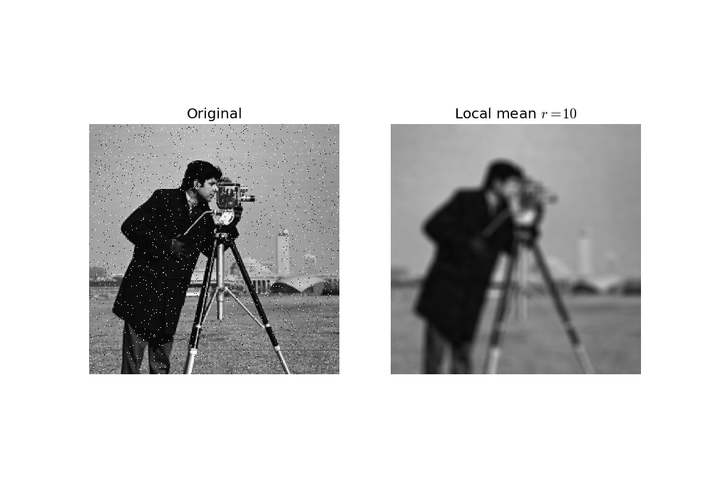
One may be interested in smoothing an image while preserving important borders (median filters already achieved this), here we use the bilateral filter that restricts the local neighborhood to pixel having a gray-level similar to the central one.
Note
A different implementation is available for color images in skimage.filter.denoise_bilateral.
from skimage.filter.rank import mean_bilateral

noisy_image = img_as_ubyte(data.camera())

bilat = mean_bilateral(noisy_image.astype(np.uint16), disk(20), s0=10, s1=10)

fig, ax = plt.subplots(2, 2, figsize=(10, 7))
ax1, ax2, ax3, ax4 = ax.ravel()

ax1.imshow(noisy_image, cmap=plt.cm.gray)
ax1.set_title('Original')
ax1.axis('off')

ax2.imshow(bilat, cmap=plt.cm.gray)
ax2.set_title('Bilateral mean')
ax2.axis('off')

ax3.imshow(noisy_image[200:350, 350:450], cmap=plt.cm.gray)
ax3.axis('off')

ax4.imshow(bilat[200:350, 350:450], cmap=plt.cm.gray)
ax4.axis('off')
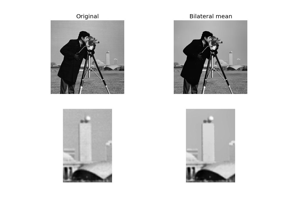
One can see that the large continuous part of the image (e.g. sky) is smoothed whereas other details are preserved.
Contrast enhancement
We compare here how the global histogram equalization is applied locally.
The equalized image [2] has a roughly linear cumulative distribution function for each pixel neighborhood. The local version [3] of the histogram equalization emphasizes every local gray-level variations.
| [2] | http://en.wikipedia.org/wiki/Histogram_equalization |
| [3] | http://en.wikipedia.org/wiki/Adaptive_histogram_equalization |
from skimage import exposure
from skimage.filter import rank

noisy_image = img_as_ubyte(data.camera())

# equalize globally and locally
glob = exposure.equalize_hist(noisy_image) * 255
loc = rank.equalize(noisy_image, disk(20))

# extract histogram for each image
hist = np.histogram(noisy_image, bins=np.arange(0, 256))
glob_hist = np.histogram(glob, bins=np.arange(0, 256))
loc_hist = np.histogram(loc, bins=np.arange(0, 256))

fig, ax = plt.subplots(3, 2, figsize=(10, 10))
ax1, ax2, ax3, ax4, ax5, ax6 = ax.ravel()

ax1.imshow(noisy_image, interpolation='nearest', cmap=plt.cm.gray)
ax1.axis('off')

ax2.plot(hist[1][:-1], hist[0], lw=2)
ax2.set_title('Histogram of gray values')

ax3.imshow(glob, interpolation='nearest', cmap=plt.cm.gray)
ax3.axis('off')

ax4.plot(glob_hist[1][:-1], glob_hist[0], lw=2)
ax4.set_title('Histogram of gray values')

ax5.imshow(loc, interpolation='nearest', cmap=plt.cm.gray)
ax5.axis('off')

ax6.plot(loc_hist[1][:-1], loc_hist[0], lw=2)
ax6.set_title('Histogram of gray values')
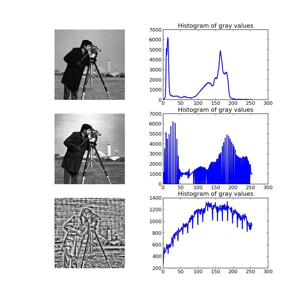
Another way to maximize the number of gray-levels used for an image is to apply a local auto-leveling, i.e. the gray-value of a pixel is proportionally remapped between local minimum and local maximum.
The following example shows how local auto-level enhances the camara man picture.
from skimage.filter.rank import autolevel

noisy_image = img_as_ubyte(data.camera())

auto = autolevel(noisy_image.astype(np.uint16), disk(20))

fig, (ax1, ax2) = plt.subplots(1, 2, figsize=[10, 7])

ax1.imshow(noisy_image, cmap=plt.cm.gray)
ax1.set_title('Original')
ax1.axis('off')

ax2.imshow(auto, cmap=plt.cm.gray)
ax2.set_title('Local autolevel')
ax2.axis('off')
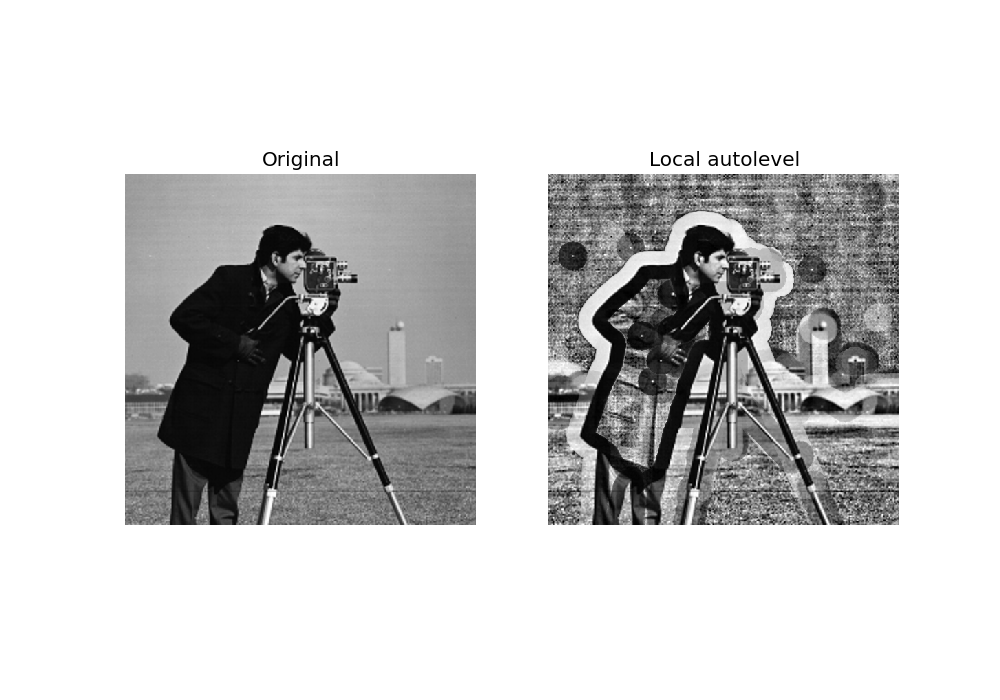
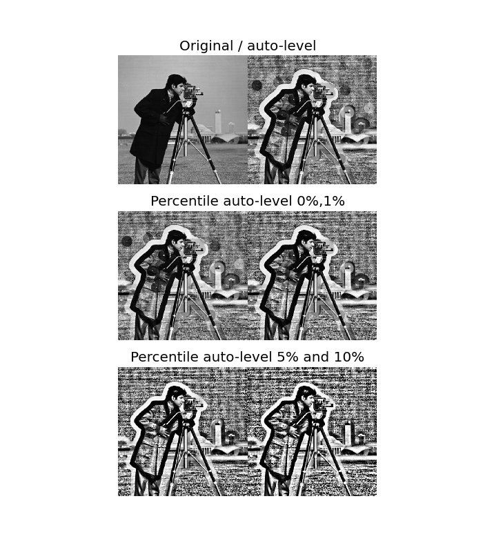
This filter is very sensitive to local outliers, see the little white spot in the left part of the sky. This is due to a local maximum which is very high comparing to the rest of the neighborhood. One can moderate this using the percentile version of the auto-level filter which uses given percentiles (one inferior, one superior) in place of local minimum and maximum. The example below illustrates how the percentile parameters influence the local auto-level result.
from skimage.filter.rank import autolevel_percentile

image = data.camera()

selem = disk(20)
loc_autolevel = autolevel(image, selem=selem)
loc_perc_autolevel0 = autolevel_percentile(image, selem=selem, p0=.00, p1=1.0)
loc_perc_autolevel1 = autolevel_percentile(image, selem=selem, p0=.01, p1=.99)
loc_perc_autolevel2 = autolevel_percentile(image, selem=selem, p0=.05, p1=.95)
loc_perc_autolevel3 = autolevel_percentile(image, selem=selem, p0=.1, p1=.9)

fig, axes = plt.subplots(nrows=3, figsize=(7, 8))
ax0, ax1, ax2 = axes
plt.gray()

ax0.imshow(np.hstack((image, loc_autolevel)), cmap=plt.cm.gray)
ax0.set_title('Original / auto-level')

ax1.imshow(
    np.hstack((loc_perc_autolevel0, loc_perc_autolevel1)), vmin=0, vmax=255)
ax1.set_title('Percentile auto-level 0%,1%')
ax2.imshow(
    np.hstack((loc_perc_autolevel2, loc_perc_autolevel3)), vmin=0, vmax=255)
ax2.set_title('Percentile auto-level 5% and 10%')

for ax in axes:
    ax.axis('off')
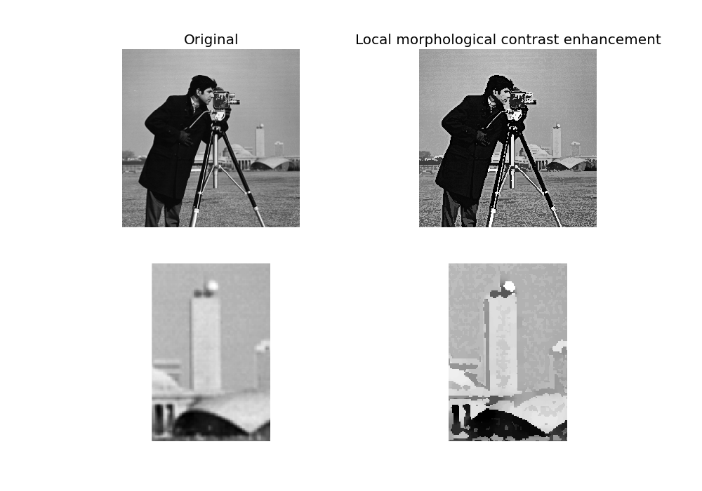
The morphological contrast enhancement filter replaces the central pixel by the local maximum if the original pixel value is closest to local maximum, otherwise by the minimum local.
from skimage.filter.rank import enhance_contrast

noisy_image = img_as_ubyte(data.camera())

enh = enhance_contrast(noisy_image, disk(5))

fig, ax = plt.subplots(2, 2, figsize=[10, 7])
ax1, ax2, ax3, ax4 = ax.ravel()

ax1.imshow(noisy_image, cmap=plt.cm.gray)
ax1.set_title('Original')
ax1.axis('off')

ax2.imshow(enh, cmap=plt.cm.gray)
ax2.set_title('Local morphological contrast enhancement')
ax2.axis('off')

ax3.imshow(noisy_image[200:350, 350:450], cmap=plt.cm.gray)
ax3.axis('off')

ax4.imshow(enh[200:350, 350:450], cmap=plt.cm.gray)
ax4.axis('off')
The percentile version of the local morphological contrast enhancement uses percentile p0 and p1 instead of the local minimum and maximum.
from skimage.filter.rank import enhance_contrast_percentile

noisy_image = img_as_ubyte(data.camera())

penh = enhance_contrast_percentile(noisy_image, disk(5), p0=.1, p1=.9)

fig, ax = plt.subplots(2, 2, figsize=[10, 7])
ax1, ax2, ax3, ax4 = ax.ravel()

ax1.imshow(noisy_image, cmap=plt.cm.gray)
ax1.set_title('Original')
ax1.axis('off')

ax2.imshow(penh, cmap=plt.cm.gray)
ax2.set_title('Local percentile morphological\n contrast enhancement')
ax2.axis('off')

ax3.imshow(noisy_image[200:350, 350:450], cmap=plt.cm.gray)
ax3.axis('off')

ax4.imshow(penh[200:350, 350:450], cmap=plt.cm.gray)
ax4.axis('off')
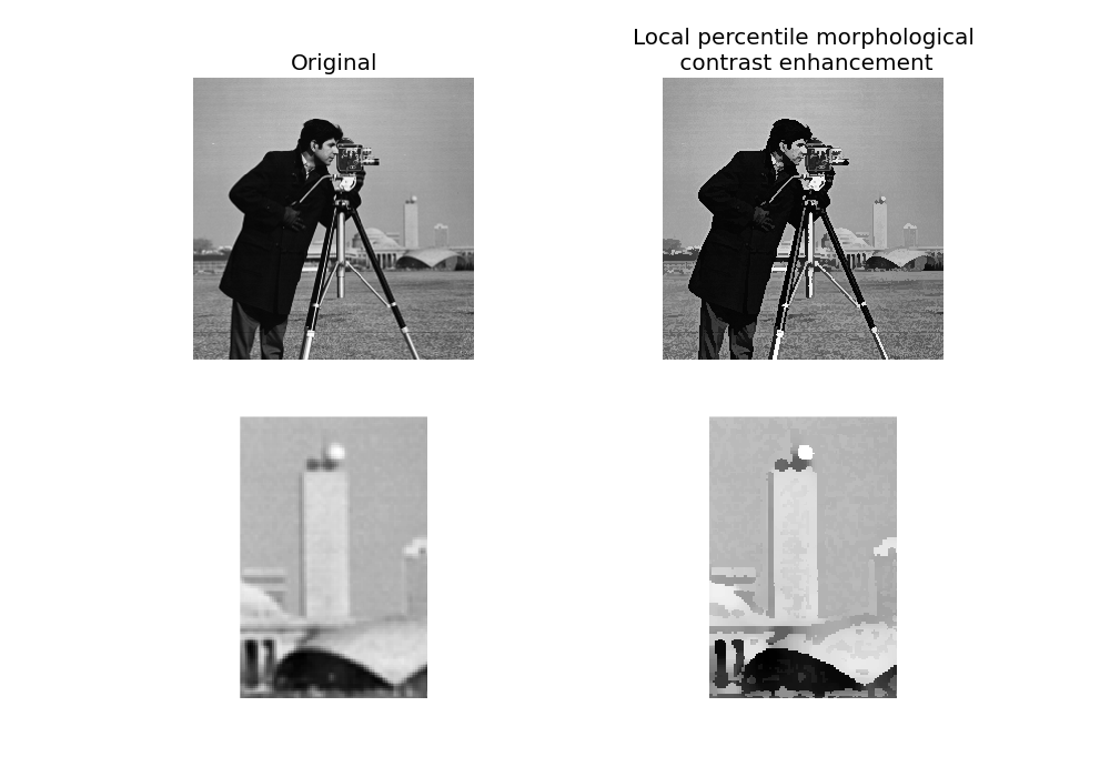
Image threshold
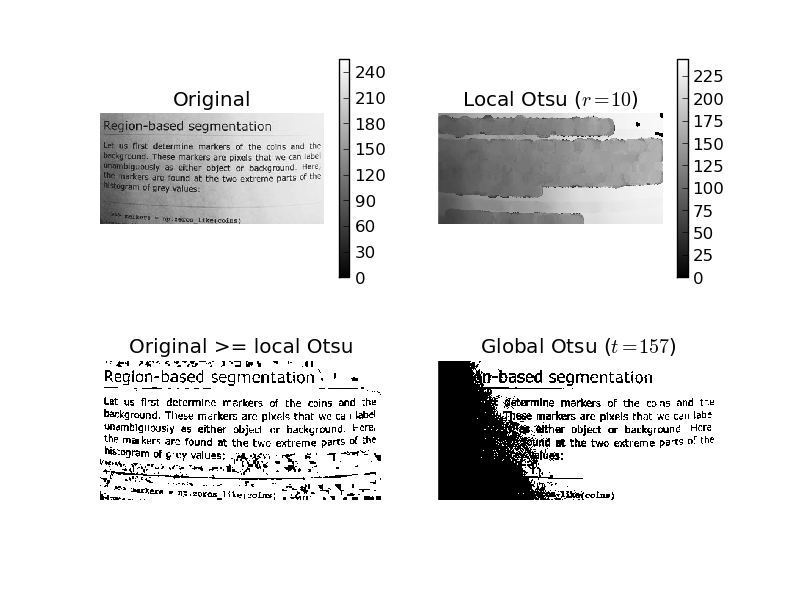
The Otsu threshold [1] method can be applied locally using the local gray- level distribution. In the example below, for each pixel, an “optimal” threshold is determined by maximizing the variance between two classes of pixels of the local neighborhood defined by a structuring element.
The example compares the local threshold with the global threshold skimage.filter.threshold_otsu.
Note
Local is much slower than global thresholding. A function for global Otsu thresholding can be found in : skimage.filter.threshold_otsu.
| [4] | http://en.wikipedia.org/wiki/Otsu’s_method |
from skimage.filter.rank import otsu
from skimage.filter import threshold_otsu

p8 = data.page()

radius = 10
selem = disk(radius)

# t_loc_otsu is an image
t_loc_otsu = otsu(p8, selem)
loc_otsu = p8 >= t_loc_otsu

# t_glob_otsu is a scalar
t_glob_otsu = threshold_otsu(p8)
glob_otsu = p8 >= t_glob_otsu

fig, ax = plt.subplots(2, 2)
ax1, ax2, ax3, ax4 = ax.ravel()

fig.colorbar(ax1.imshow(p8, cmap=plt.cm.gray), ax=ax1)
ax1.set_title('Original')
ax1.axis('off')

fig.colorbar(ax2.imshow(t_loc_otsu, cmap=plt.cm.gray), ax=ax2)
ax2.set_title('Local Otsu ($r=%d$)' % radius)
ax2.axis('off')

ax3.imshow(p8 >= t_loc_otsu, cmap=plt.cm.gray)
ax3.set_title('Original >= local Otsu' % t_glob_otsu)
ax3.axis('off')

ax4.imshow(glob_otsu, cmap=plt.cm.gray)
ax4.set_title('Global Otsu ($t=%d$)' % t_glob_otsu)
ax4.axis('off')
The following example shows how local Otsu thresholding handles a global level shift applied to a synthetic image.
n = 100
theta = np.linspace(0, 10 * np.pi, n)
x = np.sin(theta)
m = (np.tile(x, (n, 1)) * np.linspace(0.1, 1, n) * 128 + 128).astype(np.uint8)

radius = 10
t = rank.otsu(m, disk(radius))

fig, (ax1, ax2) = plt.subplots(1, 2)

ax1.imshow(m)
ax1.set_title('Original')
ax1.axis('off')

ax2.imshow(m >= t, interpolation='nearest')
ax2.set_title('Local Otsu ($r=%d$)' % radius)
ax2.axis('off')
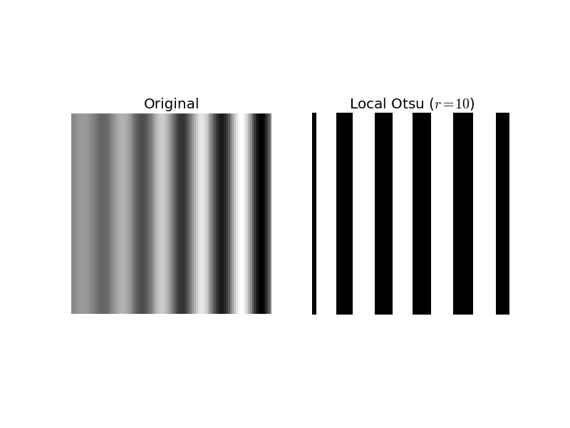
Image morphology
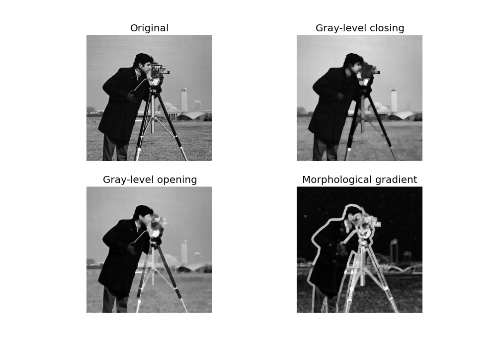
Local maximum and local minimum are the base operators for gray-level morphology.
Note
skimage.dilate and skimage.erode are equivalent filters (see below for comparison).
Here is an example of the classical morphological gray-level filters: opening, closing and morphological gradient.
from skimage.filter.rank import maximum, minimum, gradient

noisy_image = img_as_ubyte(data.camera())

closing = maximum(minimum(noisy_image, disk(5)), disk(5))
opening = minimum(maximum(noisy_image, disk(5)), disk(5))
grad = gradient(noisy_image, disk(5))

# display results
fig, ax = plt.subplots(2, 2, figsize=[10, 7])
ax1, ax2, ax3, ax4 = ax.ravel()

ax1.imshow(noisy_image, cmap=plt.cm.gray)
ax1.set_title('Original')
ax1.axis('off')

ax2.imshow(closing, cmap=plt.cm.gray)
ax2.set_title('Gray-level closing')
ax2.axis('off')

ax3.imshow(opening, cmap=plt.cm.gray)
ax3.set_title('Gray-level opening')
ax3.axis('off')

ax4.imshow(grad, cmap=plt.cm.gray)
ax4.set_title('Morphological gradient')
ax4.axis('off')
Feature extraction
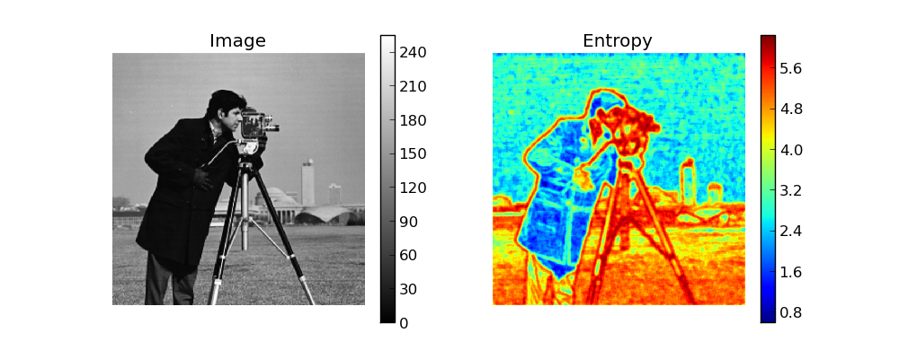
Local histograms can be exploited to compute local entropy, which is related to the local image complexity. Entropy is computed using base 2 logarithm i.e. the filter returns the minimum number of bits needed to encode local gray-level distribution.
skimage.rank.entropy returns the local entropy on a given structuring element. The following example shows applies this filter on 8- and 16-bit images.
Note
to better use the available image bit, the function returns 10x entropy for 8-bit images and 1000x entropy for 16-bit images.
from skimage import data
from skimage.filter.rank import entropy
from skimage.morphology import disk
import numpy as np
import matplotlib.pyplot as plt

image = data.camera()

fig, (ax1, ax2) = plt.subplots(1, 2, figsize=(10, 4))

fig.colorbar(ax1.imshow(image, cmap=plt.cm.gray), ax=ax1)
ax1.set_title('Image')
ax1.axis('off')

fig.colorbar(ax2.imshow(entropy(image, disk(5)), cmap=plt.cm.jet), ax=ax2)
ax2.set_title('Entropy')
ax2.axis('off')
Implementation
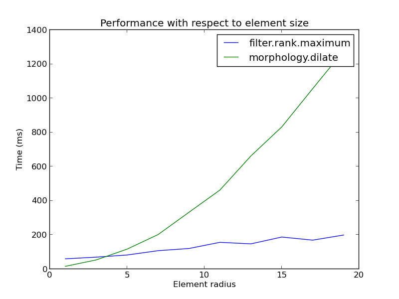
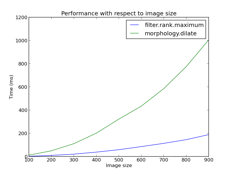
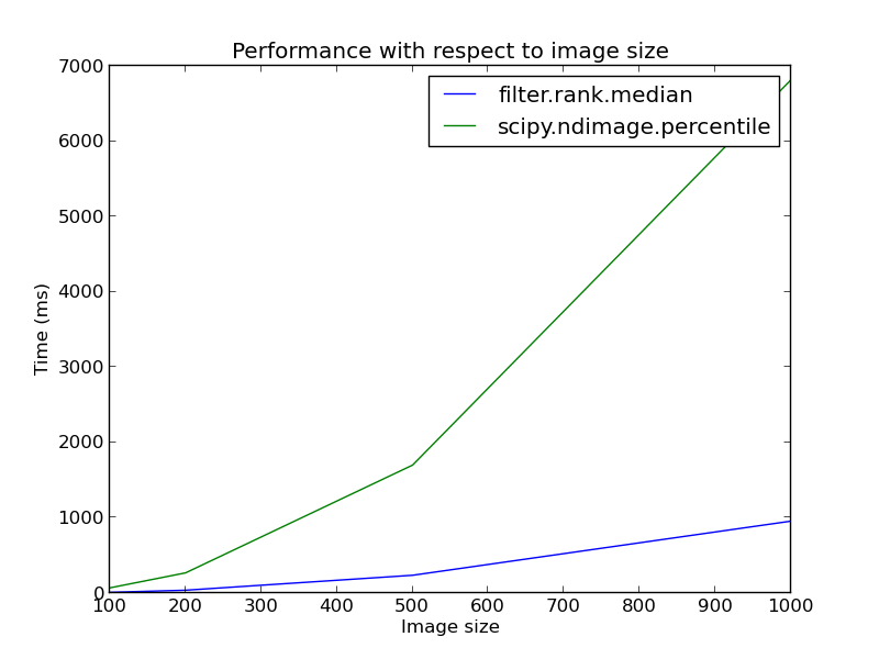
The central part of the skimage.rank filters is build on a sliding window that updates the local gray-level histogram. This approach limits the algorithm complexity to O(n) where n is the number of image pixels. The complexity is also limited with respect to the structuring element size.
In the following we compare the performance of different implementations available in skimage.
from time import time

from scipy.ndimage.filters import percentile_filter
from skimage.morphology import dilation
from skimage.filter.rank import median, maximum


def exec_and_timeit(func):
    """Decorator that returns both function results and execution time."""
    def wrapper(*arg):
        t1 = time()
        res = func(*arg)
        t2 = time()
        ms = (t2 - t1) * 1000.0
        return (res, ms)
    return wrapper


@exec_and_timeit
def cr_med(image, selem):
    return median(image=image, selem=selem)


@exec_and_timeit
def cr_max(image, selem):
    return maximum(image=image, selem=selem)


@exec_and_timeit
def cm_dil(image, selem):
    return dilation(image=image, selem=selem)


@exec_and_timeit
def ndi_med(image, n):
    return percentile_filter(image, 50, size=n * 2 - 1)
Comparison between
- filter.rank.maximum
- morphology.dilate
on increasing structuring element size:
a = data.camera()

rec = []
e_range = range(1, 20, 2)
for r in e_range:
    elem = disk(r + 1)
    rc, ms_rc = cr_max(a, elem)
    rcm, ms_rcm = cm_dil(a, elem)
    rec.append((ms_rc, ms_rcm))

rec = np.asarray(rec)

fig, ax = plt.subplots()
ax.set_title('Performance with respect to element size')
ax.set_ylabel('Time (ms)')
ax.set_xlabel('Element radius')
ax.plot(e_range, rec)
ax.legend(['filter.rank.maximum', 'morphology.dilate'])
and increasing image size:
r = 9
elem = disk(r + 1)

rec = []
s_range = range(100, 1000, 100)
for s in s_range:
    a = (np.random.random((s, s)) * 256).astype(np.uint8)
    (rc, ms_rc) = cr_max(a, elem)
    (rcm, ms_rcm) = cm_dil(a, elem)
    rec.append((ms_rc, ms_rcm))

rec = np.asarray(rec)

fig, ax = plt.subplots()
ax.set_title('Performance with respect to image size')
ax.set_ylabel('Time (ms)')
ax.set_xlabel('Image size')
ax.plot(s_range, rec)
ax.legend(['filter.rank.maximum', 'morphology.dilate'])
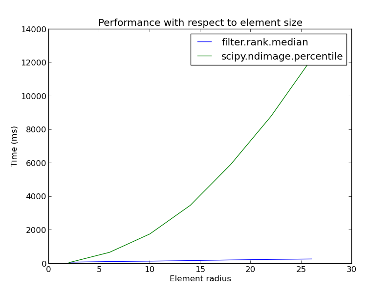
Comparison between:
- filter.rank.median
- scipy.ndimage.percentile
on increasing structuring element size:
a = data.camera()

rec = []
e_range = range(2, 30, 4)
for r in e_range:
    elem = disk(r + 1)
    rc, ms_rc = cr_med(a, elem)
    rndi, ms_ndi = ndi_med(a, r)
    rec.append((ms_rc, ms_ndi))

rec = np.asarray(rec)

fig, ax = plt.subplots()
ax.set_title('Performance with respect to element size')
ax.plot(e_range, rec)
ax.legend(['filter.rank.median', 'scipy.ndimage.percentile'])
ax.set_ylabel('Time (ms)')
ax.set_xlabel('Element radius')
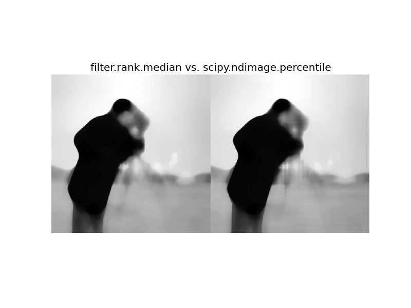
Comparison of outcome of the three methods:
fig, ax = plt.subplots()
ax.imshow(np.hstack((rc, rndi)))
ax.set_title('filter.rank.median vs. scipy.ndimage.percentile')
ax.axis('off')
and increasing image size:
r = 9
elem = disk(r + 1)

rec = []
s_range = [100, 200, 500, 1000]
for s in s_range:
    a = (np.random.random((s, s)) * 256).astype(np.uint8)
    (rc, ms_rc) = cr_med(a, elem)
    rndi, ms_ndi = ndi_med(a, r)
    rec.append((ms_rc, ms_ndi))

rec = np.asarray(rec)

fig, ax = plt.subplots()
ax.set_title('Performance with respect to image size')
ax.plot(s_range, rec)
ax.legend(['filter.rank.median', 'scipy.ndimage.percentile'])
ax.set_ylabel('Time (ms)')
ax.set_xlabel('Image size')
plt.show()
Python source code: download (generated using skimage 0.10dev)
IPython Notebook: download (generated using skimage 0.10dev)
